Using BiVariAn • BiVariAn

library(BiVariAn)

Using BiVariAn solves several different problems, each one described in its corresponding function.

Functions

There are currently several groups of functions available:

Database oriented

encode_factors
fix_mixed_cols

Plotting oriented

theme_serene
theme_serene_void
auto_bar_categ
auto_bar_cont
auto_viol_cont
auto_bp_cont
auto_corr_cont
auto_dens_cont
auto_pie_categ

Univariate and bivariate analyses

auto_shapiro_raw
dichotomous_2k_2sid
continuous_2g
continuous_2g_pair
continuous_corr_test
continuous_multg
continuous_multg_rm

Regression analyses

step_bw_p
step_bw_firth
logistf_summary
ss_multreg

Usage examples

Suppose we want to start an analysis of a dataset with a large number of variables. Typically, we would have to run normality tests, which would mean writing one line of code for every variable. As an example, we will use the penguins dataset available in the palmerpenguins package.

data(penguins)

dat <- penguins

Normality

If we inspect the dataset we have 8 variables with 344 observations. Among these variables there are 5 numeric variables (one of them representing years), which would mean writing normality test code for each of them.

shapiro.test(dat$bill_len)
#> 
#>  Shapiro-Wilk normality test
#> 
#> data:  dat$bill_len
#> W = 0.97485, p-value = 1.12e-05

More advanced users might consider writing a loop or using helper functions such as lapply to evaluate all variables through a list (or similar approaches).

cont_var <- c("bill_len", "bill_dep", "flipper_len", "body_mass")

lapply(dat[cont_var], function(x) shapiro.test(x))
#> $bill_len
#> 
#>  Shapiro-Wilk normality test
#> 
#> data:  x
#> W = 0.97485, p-value = 1.12e-05
#> 
#> 
#> $bill_dep
#> 
#>  Shapiro-Wilk normality test
#> 
#> data:  x
#> W = 0.97258, p-value = 4.419e-06
#> 
#> 
#> $flipper_len
#> 
#>  Shapiro-Wilk normality test
#> 
#> data:  x
#> W = 0.95155, p-value = 3.54e-09
#> 
#> 
#> $body_mass
#> 
#>  Shapiro-Wilk normality test
#> 
#> data:  x
#> W = 0.95921, p-value = 3.679e-08

With BiVariAn we can solve this problem (and improve the display of the results) by using the auto_shapiro_raw function.

auto_shapiro_raw(data = dat)

Variable	p_shapiro	Normality
bill_len	<0.001*	Non-normal
bill_dep	<0.001*	Non-normal
flipper_len	<0.001*	Non-normal
body_mass	<0.001*	Non-normal
year	<0.001*	Non-normal

Do we want a data frame instead of a flextable? We can do that with the flextableformat argument (which is used in most functions).

shapirores <- auto_shapiro_raw(
  data = dat, 
  flextableformat = FALSE
)

shapirores
#>                Variable p_shapiro  Normality
#> bill_len       bill_len   <0.001* Non-normal
#> bill_dep       bill_dep   <0.001* Non-normal
#> flipper_len flipper_len   <0.001* Non-normal
#> body_mass     body_mass   <0.001* Non-normal
#> year               year   <0.001* Non-normal

Bivariate analyses

After checking normality, the next natural step is to apply bivariate tests, but again we would have to write separate code for each test. For example, if we wanted to compare variables across sexes, we would write something like this for every variable.

Note

The normality analysis showed a non normal distribution, so ideally at this stage we would not apply parametric tests. For now, we will continue as if we needed to perform a t test, only to illustrate the workflow.

# First we would evaluate homoscedasticity
car::leveneTest(
  dat$bill_len, 
  group = dat$sex,
  center = "median"
)
#> Levene's Test for Homogeneity of Variance (center = "median")
#>        Df F value  Pr(>F)  
#> group   1  2.8244 0.09378 .
#>       331                  
#> ---
#> Signif. codes:  0 '***' 0.001 '**' 0.01 '*' 0.05 '.' 0.1 ' ' 1

# Then we apply the t test
t.test(dat$bill_len)
#> 
#>  One Sample t-test
#> 
#> data:  dat$bill_len
#> t = 148.78, df = 341, p-value < 2.2e-16
#> alternative hypothesis: true mean is not equal to 0
#> 95 percent confidence interval:
#>  43.34125 44.50261
#> sample estimates:
#> mean of x 
#>  43.92193

Doing this for every variable quickly becomes an iterative and repetitive process, and in addition we would need to write separate code to report mean differences with their corresponding tests.

With BiVariAn we can avoid this by using the continuous_2g function.

continuous_2g(
  data = dat,
  groupvar = "sex"
)

Variable	P_Shapiro_Resid	P_Levene	P_T_Test	Var_Equal	P_Mann_Whitney	Diff_Means	CI_Lower	CI_Upper	Significant_test
bill_len	<0.001*	0.09	<0.001*	true	<0.001*	-3.76	-4.87	-2.65	Mann-W-U test
bill_dep	<0.001*	0.69	<0.001*	true	<0.001*	-1.47	-1.86	-1.07	Mann-W-U test
flipper_len	<0.001*	0.04	<0.001*	false	<0.001*	-7.14	-10.06	-4.22	Mann-W-U test
body_mass	<0.001*	0.01	<0.001*	false	<0.001*	-683.41	-840.58	-526.25	Mann-W-U test
year	<0.001*	1.00	0.99323	true	0.99373	0.00	-0.17	0.18	None

Customizing the output

Similarly, we can use the flextableformat argument to obtain a data frame.

continuous_2g(
  data = dat,
  groupvar = "sex",
  flextableformat = FALSE
)
#>      Variable P_Shapiro_Resid P_Levene P_T_Test Var_Equal P_Mann_Whitney
#> 1    bill_len         <0.001*  0.09378  <0.001*      TRUE        <0.001*
#> 2    bill_dep         <0.001*  0.68955  <0.001*      TRUE        <0.001*
#> 3 flipper_len         <0.001*  0.04011  <0.001*     FALSE        <0.001*
#> 4   body_mass         <0.001*  0.01435  <0.001*     FALSE        <0.001*
#> 5        year         <0.001*  0.99834  0.99323      TRUE        0.99373
#>   Diff_Means   CI_Lower   CI_Upper Significant_test
#> 1   -3.75779   -4.86656   -2.64903    Mann-W-U test
#> 2   -1.46562   -1.86021   -1.07103    Mann-W-U test
#> 3   -7.14232  -10.06481   -4.21982    Mann-W-U test
#> 4 -683.41180 -840.57826 -526.24533    Mann-W-U test
#> 5    0.00076   -0.17478    0.17630             None

However, we can also add labels to the variables using the table1::label() function from the table1 package.

library(table1)
#> 
#> Attaching package: 'table1'
#> The following objects are masked from 'package:base':
#> 
#>     units, units<-

table1::label(dat$sex)        <- "Sex"
table1::label(dat$bill_len)   <- "Bill length"
table1::label(dat$bill_dep)   <- "Bill depth"

And we obtain a nicely labeled table.

continuous_2g(
  data = dat,
  groupvar = "sex"
)

Variable	P_Shapiro_Resid	P_Levene	P_T_Test	Var_Equal	P_Mann_Whitney	Diff_Means	CI_Lower	CI_Upper	Significant_test
Bill length	<0.001*	0.09	<0.001*	true	<0.001*	-3.76	-4.87	-2.65	Mann-W-U test
Bill depth	<0.001*	0.69	<0.001*	true	<0.001*	-1.47	-1.86	-1.07	Mann-W-U test
flipper_len	<0.001*	0.04	<0.001*	false	<0.001*	-7.14	-10.06	-4.22	Mann-W-U test
body_mass	<0.001*	0.01	<0.001*	false	<0.001*	-683.41	-840.58	-526.25	Mann-W-U test
year	<0.001*	1.00	0.99323	true	0.99373	0.00	-0.17	0.18	None

Do we want a title row that indicates the grouping variable? We can add it with the caption argument.

continuous_2g(
  data = dat,
  groupvar = "sex",
  caption = TRUE
)

Sex
Variable	P_Shapiro_Resid	P_Levene	P_T_Test	Var_Equal	P_Mann_Whitney	Diff_Means	CI_Lower	CI_Upper	Significant_test
Bill length	<0.001*	0.09	<0.001*	true	<0.001*	-3.76	-4.87	-2.65	Mann-W-U test
Bill depth	<0.001*	0.69	<0.001*	true	<0.001*	-1.47	-1.86	-1.07	Mann-W-U test
flipper_len	<0.001*	0.04	<0.001*	false	<0.001*	-7.14	-10.06	-4.22	Mann-W-U test
body_mass	<0.001*	0.01	<0.001*	false	<0.001*	-683.41	-840.58	-526.25	Mann-W-U test
year	<0.001*	1.00	0.99323	true	0.99373	0.00	-0.17	0.18	None

Important

To use the caption argument it is mandatory that flextableformat is TRUE; otherwise an error will be raised.

Graphical representation

The next step would be to create graphical representations. Again, if we want to use ggplot2 we would write separate code for every plot (which implies multiple lines of code that can become tedious if we want extensive customization).

Let us create a boxplot to represent the comparison of flipper_len across the sex variable.

library(tidyr)
library(dplyr)
#> 
#> Attaching package: 'dplyr'
#> The following objects are masked from 'package:stats':
#> 
#>     filter, lag
#> The following objects are masked from 'package:base':
#> 
#>     intersect, setdiff, setequal, union
library(ggplot2)

dat_comp <- dat %>% 
  drop_na(sex) # We remove the NAs from the sex variable

ggplot(
  data = dat_comp,
  mapping = aes(
    x = sex,
    y = flipper_len
  )
) + 
  geom_boxplot() + 
  labs(
    x = "Sex",
    y = "Flipper length"
  ) + 
  theme_classic()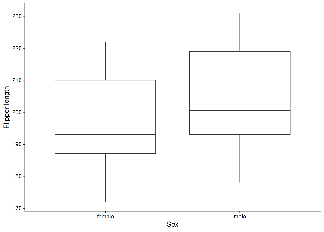

Repeating this for every variable implies multiple lines of code. For this reason, the auto_bp_cont function can help streamline the workflow.

We simply call the function and store its output in an object. This object is a list, so we can select the specific plot we want to display or include in our report.

graphs <- auto_bp_cont(
  data = dat_comp, 
  groupvar = "sex"
)

graphs$flipper_len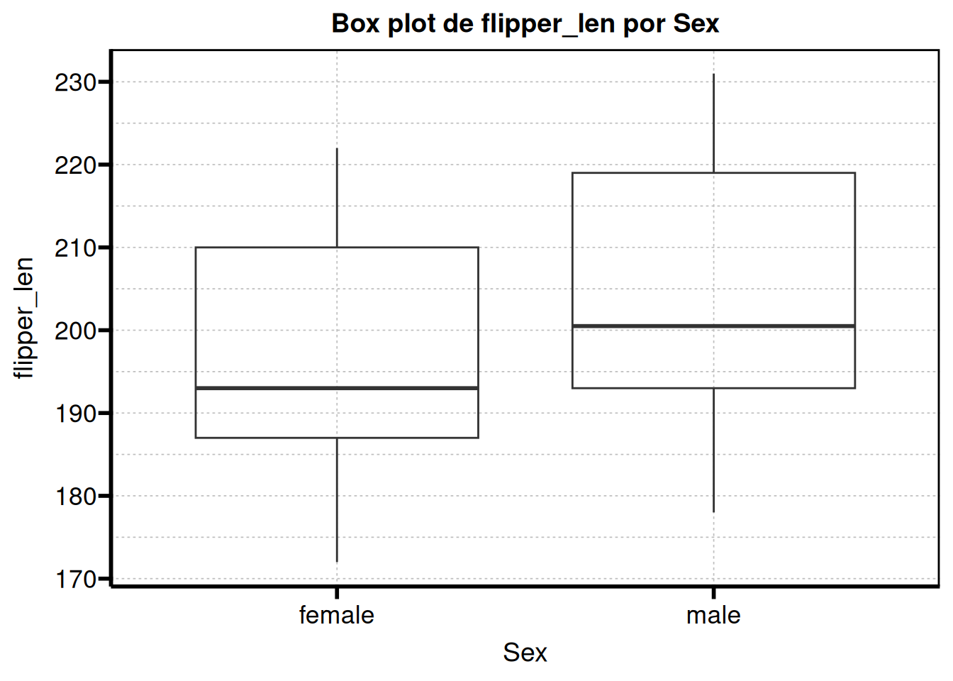

If you remember, we previously assigned labels using table1::label(). The good news is that these labels can also be used for the plots.

table1::label(dat_comp$sex)         <- "Sex"
table1::label(dat_comp$flipper_len) <- "Flipper length"

graphs <- auto_bp_cont(
  data = dat_comp, 
  groupvar = "sex"
)

graphs$flipper_len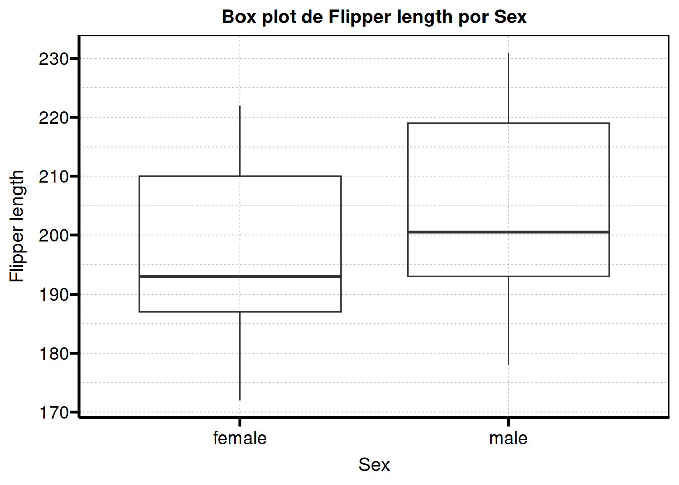

At this point we have everything we need to build our report.

Special mentions

As a special mention, there are some useful helper functions for regression analysis. For example, the step_bw_p function helps with the tedious iterative process of simplifying regression models by stepwise backward selection based on a p value threshold, and the step_bw_firth function performs the same process for models fitted with logistf::logistf().

If we fit a model with our dataset, we obtain something like this:

model_reg <- glm(
  sex ~ species + island + bill_len + bill_dep + flipper_len + body_mass, 
  data = dat, 
  family = binomial()
)

step_bw_p(model_reg)
#> 
#> Initial model: sex ~ species + island + bill_len + bill_dep + flipper_len + body_mass 
#> Analysis of Deviance Table (Type II tests)
#> 
#> Response: sex
#>             LR Chisq Df Pr(>Chisq)    
#> species       32.685  2  7.991e-08 ***
#> island         1.061  2     0.5882    
#> bill_len      32.923  1  9.588e-09 ***
#> bill_dep      35.316  1  2.803e-09 ***
#> flipper_len    0.304  1     0.5815    
#> body_mass     50.238  1  1.362e-12 ***
#> ---
#> Signif. codes:  0 '***' 0.001 '**' 0.01 '*' 0.05 '.' 0.1 ' ' 1
#> 
#> Removing island (p = 0.5882)
#> Analysis of Deviance Table (Type II tests)
#> 
#> Response: sex
#>             LR Chisq Df Pr(>Chisq)    
#> species       31.895  2  1.186e-07 ***
#> bill_len      33.097  1  8.769e-09 ***
#> bill_dep      34.748  1  3.752e-09 ***
#> flipper_len    0.189  1     0.6638    
#> body_mass     51.667  1  6.575e-13 ***
#> ---
#> Signif. codes:  0 '***' 0.001 '**' 0.01 '*' 0.05 '.' 0.1 ' ' 1
#> 
#> Removing flipper_len (p = 0.6638)
#> Analysis of Deviance Table (Type II tests)
#> 
#> Response: sex
#>           LR Chisq Df Pr(>Chisq)    
#> species     32.590  2  8.378e-08 ***
#> bill_len    33.727  1  6.343e-09 ***
#> bill_dep    36.486  1  1.538e-09 ***
#> body_mass   58.852  1  1.700e-14 ***
#> ---
#> Signif. codes:  0 '***' 0.001 '**' 0.01 '*' 0.05 '.' 0.1 ' ' 1
#> 
#> No eliminable terms above p_threshold. Stopping.
#> $final_model
#> 
#> Call:  glm(formula = sex ~ species + bill_len + bill_dep + body_mass, 
#>     family = binomial(), data = dat)
#> 
#> Coefficients:
#>      (Intercept)  speciesChinstrap     speciesGentoo          bill_len  
#>       -76.093935         -6.897694         -7.875212          0.620082  
#>         bill_dep         body_mass  
#>         1.643613          0.005962  
#> 
#> Degrees of Freedom: 332 Total (i.e. Null);  327 Residual
#>   (11 observations deleted due to missingness)
#> Null Deviance:       461.6 
#> Residual Deviance: 127.3     AIC: 139.3
#> 
#> $steps
#>            Step
#> 1       Initial
#> 2      - island
#> 3 - flipper_len
#>                                                                    Formula
#> 1 "sex ~ species + island + bill_len + bill_dep + flipper_len + body_mass"
#> 2          "sex ~ species + bill_len + bill_dep + flipper_len + body_mass"
#> 3                        "sex ~ species + bill_len + bill_dep + body_mass"
#> 
#> attr(,"class")
#> [1] "step_bw"

In practice, this removes the need to manually perform three backward selection steps (which would otherwise require typing the full model each time or using helpers such as reformulate).

We can also store the output in an object:

step_res <- step_bw_p(
  model_reg, 
  trace = FALSE # To avoid printing the process in the console
)

step_res$steps       # Data frame of the steps involved
#>            Step
#> 1       Initial
#> 2      - island
#> 3 - flipper_len
#>                                                                    Formula
#> 1 "sex ~ species + island + bill_len + bill_dep + flipper_len + body_mass"
#> 2          "sex ~ species + bill_len + bill_dep + flipper_len + body_mass"
#> 3                        "sex ~ species + bill_len + bill_dep + body_mass"
step_res$final_model # Final model after all iterations
#> 
#> Call:  glm(formula = sex ~ species + bill_len + bill_dep + body_mass, 
#>     family = binomial(), data = dat)
#> 
#> Coefficients:
#>      (Intercept)  speciesChinstrap     speciesGentoo          bill_len  
#>       -76.093935         -6.897694         -7.875212          0.620082  
#>         bill_dep         body_mass  
#>         1.643613          0.005962  
#> 
#> Degrees of Freedom: 332 Total (i.e. Null);  327 Residual
#>   (11 observations deleted due to missingness)
#> Null Deviance:       461.6 
#> Residual Deviance: 127.3     AIC: 139.3